Friday, October 23, 2009

A silent death of the Horizontal no Free Lunch theorem

The only reply I got for my concerns regarding W. Dembski's and R. Marks's article The Search for a Search - and its Horizontal No Free Lunch theorem - was an email from R. Marks, stating that he'd look into it.
Now, two weeks later, R. Marks took the article from his list of publications. The Evolutionary Informatics lab has still an announcement, basically the abstract of the article:
Many searches are needle-in-the-haystack problems, looking for small targets in large spaces. In such cases, blind search can stand no hope of success. Success, instead, requires an assisted search. But whence the assistance required for a search to be successful? To pose the question this way suggests that successful searches do not emerge spontaneously but need themselves to be discovered via a search. The question then naturally arises whether such a higher-level “search for a search” is any easier than the original search. We prove two results: (1) The Horizontal No Free Lunch Theorem, which shows that average relative performance of searches never exceeds unassisted or blind searches. (2) The Vertical No Free Lunch Theorem, which shows that the difficulty of searching for a successful search increases exponentially compared to the difficulty of the original search.
The given link doesn't lead to the article any longer, but to their earlier opus Conservation of Information in Search - neither the term vertical nor the term horizontal appear in this article.

In his first podcast with Casey Luskin, W. Dembski promised that this article was something like a nail to the coffin of evolution. I assume that W. Dembski will explain how he was wrong with this assessment in his next interview...

One if by land, and two if by sea...

Or, in the Intelligent Design version: Two lanterns contain the same information as one lantern, ergo, they come by land...

Thursday, October 22, 2009

Horizontal No Free Lunch Theorem

You keep using that word. I do not think it means what you think it means
Inigo Montoya


In their upcoming paper The Search for a Search: Measuring the Information Cost of Higher Level Search W. Dembski and R.Marks introduce a Horizontal No Free Lunch Theorem.

At Uncommon Descent, I tried to reach W. Dembski with the following post which is - of course - awaiting moderation at the moment.

The Horizontal No free Lunch Theorem doesn't work for a search of length m > 1 for a target T ⊆ Ω:

Let Ω be a finite search-space, T ⊆ Ω the target - a non-empty subset of Ω. A search is a (finite) sequence of Ω-valued random variables (φ1, φ2, ..., , φm). A search is successful, if φn ∈ T for one n, 1 ≤ n ≤ m.

I suppose we do agree here. Now, we look at a search Φ as a Ωm-valued random variable, i.e., Φ := (φ1, φ2, ..., , φm).

When is it successful? If we are still looking for a T ⊆ Ω we can say that we found T during our search if

Φ ∈ Ωm \ (Ω \ T)m

Let's define Θ as the subspace of Ωm which exists from the representations of targets in Ω, i.e.,

Θ := {Ωm \ (Ω \ T)m|T non-empty subset of Ω}

Obviously, Θ is much smaller than Ωm.

But this Θ is the space of feasible targets. And if you take an exhaustive partition of Θ instead of Ωm in Theorem III.1 Horizontal No Free Lunch, you'll find that you can indeed have positive values for the active entropy as defined in the same theorem.

But that's not much of a surprise, as random sampling without repetition works better than random sampling with repetition.

But if you allow T to be any subset of Ωm, your results get somewhat trivial, as you are now looking at m independent searches of length 1 for different targets.

The searches which you state as examples in this paper and the previous one all work with a fixed target, i.e., elements of Θ. You never mention the possibility that the target changes between the steps of the search (one possible interpretation of taking arbitrary subsets of Ωm into account).

So, I'm faced with two possibilities:
  1. You didn't realize the switch from stationary targets to moving ones when you introduced searching for an arbitrary subset of Ωm
  2. You realized this switch to a very different concept, but chose not to stress the point.

Tuesday, October 20, 2009

W. Dembski's and R. Marks's The Search for a Search and my major problem with it

William Dembski and Robert Marks announced a new paper The Search for a Search: Measuring the Information Cost of Higher Level Search (draft) which should appear in a peer-reviewed journal at any moment.

My problem: When I read the term search for a target without any qualifier, I imagine that
  1. the target is fix
  2. the search is over when the target is found the first time


A model for this: a game of Battleship against a random generator with this additional rules:
  1. all ships are of size one
  2. you don't know how many ships there are
  3. the game is over with the first hit


So, if your search space is Ω then there are 2|&Omega| - 1 different targets.

But with this kind of target, the math of W. Dembski's and R. Marks's paper doesn't work: They claim that you can't find a strategy for that works better on average than random search. In the Battleship example: there is no better strategy than shooting at random each turn until your first hit. But this is obviously wrong: A better strategy is not to hit a square twice.

But W. Dembski and R. Marks proved their claim - how so? Well, they redefined the concept of target. The altered rules for the Battleship:
  1. the position and the number of the ships changes each round
  2. to succeed, you have to hit a ship each round


For this version - and not for the one above - they proved all their results. The problem: That's not search as we now it...

The technical details: In section III, B, they formalize a search
Suppose now ­ Ω denotes an arbitrary search space. In general, assume ­Ω is a compact metric space with metric D, though for most theorems and calculations assume ­Ω is finite (in which case D is a discrete metric). Let X1, X2,...,Xn denote ­Ω-valued random variables that are independent and identically distributed with uniform probability distribution U. X1, X2,...,Xm therefore represents a blind search of ­Ω. Next, let Y1, Y2,...,Ym denote ­Ω-valued random variables that are arbitrarily distributed. X1, X2,...,Xn therefore characterizes an assisted search of ­Ω.


That's our first version of Battleship - I've no problem with this section. But the next paragraph states
If we now let ­Ωm denote the m-fold Cartesian product of Ω­, then X1, X2,...,Xm and Y1, Y2,...,Ym are ­m-valued random variables. Because the uniform probability on ­­Ωm is just the m-fold product measure of U, X1, X2,...,Xm) is uniformly distributed on
­ = Ωm. Thus, by attending solely to the probabilistic
structure of searches, we represent the blind search := (X1, X2,...,Xm) as having a m-dimensional uniform distribution with respect to a metric D~ that suitably extends to the metric D on Ω­. Moreover, we represent the assisted search := (Y1, Y2,...,Ym ), in searching for an arbitrary subset of , as having distribution on .
But all these tildes are superfluous. Dropping them, we see that the probabilistic connection between a blind search and an assisted search can be entirely characterized in terms of a search space ­, a metric D that induces a compact topology on ­Ω, a target T included
in ­Ω, a uniform probability measure U on ­ induced by D, and an arbitrary probability measure φ on ­Ω. U represents the probabilistic structure of a blind search, and φ represents the probabilistic structure of an assisted search.


Now, is a subset of Ωm - and there are 2|Ω| m -1 non-empty subsets! A successful search means that , i.e., Yn ∈ Tn for all 1 ≤ n ≤ m. So, a stationary target would be not represented by

Tn

as one may naively expect, but by

T×Ω×...×Ω
∪ Ω×T×Ω×...×Ω
∪ Ω×Ω×T×Ω×...×Ω
∪...
∪ &Omega×Ω×...×&Omega×T

but most of the targets don't fit this pattern.

Of course you can claim that knowing that you target doesn't move is additional information. But I haven't encountered a definition of search which expects you to be right on target each time...

P.S.: I tried to reach R. Marks via email - and I left an entry at W. Dembski's blog...

P.P.S.: some details.

Saturday, October 17, 2009

I wrote a letter to W. Dembski and R. Marks

After reading their article Conservation of Information in Search:
Measuring the Cost of Success
in some detail, I decided to write to W. Dembski and R. Marks, just to hint them to some minor miscalculations: So, they have the chance to get at least the math straight in their peer-reviewed paper.

At uncommondescent.com, I tried to draw attendance of Willima Dembski to two minor errors in your IEEE paper ''Conservation of Information in Search – Measuring the Cost of Success'':

Could you correct the sign errors in equation (27) and on page 1057, left column, for Q?

More problematic is the next line: you speak about the active information per query, but you calculate the active information per generation, as you drop the factor -2 from Q ~ -2log(L)/log(1-2µ) and so reach

I+ ~ L/log(L) * log(1-2µ) instead of
I+ ~ L/(2*log(L)) * log(1-2µ).

So, I+ should be µ*L/ln(L) and not 2*µ*L/ln(L).

(I stumbled upon this when I calculated my approximation I+ ~ µ*L/H_((1-b)L) for the average number of queries Q ~ H_((1-b)L)/µ )

And there is a little problem with Fig. 2: all the paths seem to start with no correct bits at all - while the math in ch. III-2 assumes that half of the bits are correct.

Let L=100, µ=0.00005:

1. if you use b(eta) = .5 (as in your calculation) Q ~ 92,100 and I+ ~ 0.00109. Then, you should take other paths for your pic

2. if you use b(eta) = 0 (as in you figure) Q ~ 106,000 and I+ ~ 0.000943

The number in your text is I+ ~0.0022. That's wrong in any case.


Yours
Di***** Eb**


Don't get me wrong: I don't want to be just nit-picking. One sign error is no big deal, an even number of sign errors cancels itself out :-)
And the factor two? It's at least the same order of magnitude. (And no one know what magnitude is to be expected for active information, so even a factor 100 would not have been easily spotted). And I didn't mention all the inaccuracies in their references' section....

Monday, October 12, 2009

Code I'm not proud of...

I was asked for the code I used to make my little pics. Well, it's not pretty, it's just a few functions in R. For example:

weasel.matrix.solo <- function(target.length=5, alphabet.length=27,mut.prob=.04,mut.effect=FALSE){
if(mut.effect) mut.prob <- alphabet.length*mut.prob/(alphabet.length-1)
M <- matrix(integer((target.length+1)*(target.length+1)),nrow=target.length+1)
for(k in 1:(target.length)){
verschlechtert <- integer(2*target.length+2)
verbessert <- verschlechtert
verschlechtert[1:k + target.length +1] <- dbinom(0:(k-1),k-1,mut.prob*(alphabet.length-1)/alphabet.length)
verbessert[1:(target.length+2-k) + target.length + 1] <- dbinom(0:(target.length+1-k),(target.length+1-k),mut.prob/alphabet.length)
for(kk in 1:(target.length+1)){
M[k,kk] <-sum( verbessert[(0:target.length) + target.length+3-k]*verschlechtert[0:target.length +target.length+3-kk])
}
}
M[target.length+1,target.length+1] <- 1
return(M)
}


This creates a transition matrix for Dawkins's algorithm with a single child. target.length is the length of the target phrase, alphabet.length is self-explaining, mut.prob is the probability with which a letter is mutated: if mut.effect==FALSE, such a mutation has no effect with probability 1/N, i.e., it's a change to the same letter :-)


weasel.matrix.cum <- function(M, pop.size = 10){
target.length <- dim(M)[1]-1
M1 <- M
for(k in 1:(target.length)){
M1[k,] <- cumsum(M[k,])
}
M1 <- M1^pop.size
for(k in 1:(target.length))
M1[k,] <- M1[k,] - c(0,M1[k,-target.length-1])
return(M1)
}

creates a transition matrix for a whole population of size pop.size, given a transition matrix M for a single-child process.

The last thing which is needed is this little snippet:
erw.exakt <- function(M,start.vektor){

M.size <- dim(M)[1]
M <- M[-M.size, -M.size]
M <- solve(diag(M.size-1)-M)
M <- apply(M,1,sum)
return(sum(start.vektor[1:(M.size-1)] * M))
}

Here, the expected value of generations for a transition matrix M is calculated, using a initial distribution for start.vektor (mostly Bin(target.length,mut.prob) distributed - or just the first unit vector).

If I ever prettify this code, I'll take Tom English on his generous offer to put it somewhere on the net.

Another approach

I completed this little project here.

I thought about different ways to present my ideas on W. Dembski's and R. Marks's article Conservation of Information in Search: Measuring the Cost of Success, and tried a few out in the last posts. The section which I'm interested in is the description of three evolutionary algorithms they give on pp. 1055-1057. Here's another approach for III E - G:


Original TextAnnotiations
E. Partitioned Search
Partitioned search [12] is a “divide and conquer” procedure best introduced by example.The name partitioned search seems to be an invention of R. Marks and W. Dembski. The reference is made to Dawkins's book The Blind Watchmaker in which the phrase can't be found. (See Tom English's blog)
Consider the L = 28 character phrase
METHINKS∗IT∗IS∗LIKE∗A∗WEASEL. (19)
This is indeed a phrase which is used in Dawkins's book - in an algorithm with which Dawkins explained the idea of cumulative selection.
Suppose that the result of our first query of L =28 characters is

SCITAMROFN∗IYRANOITULOVESAM. (20)
An example of the egregious humorous skills of Dembski and Marks: backwards, we get:
mas*evolutionaryi*nformatics
That's no problem, as the first phrase of the algorithm can be arbitrarily chosen
Two of the letters {E, S} are in the correct position. They are
shown in a bold font. In partitioned search, our search for these
letters is finished.
At least, that's the way Dembski's and Marks's search works
For the incorrect letters, we select 26 new letters and obtain

OOT∗DENGISEDESEHT∗ERA∗NETSIL. (21)
listen*are*thesedesigned*too
hilarious. And an sign that we don't see the output of an actual program, but something imagined to be a run of their algorithm. BTW, the fitness function would have to encode the position of the correct letters, and the possible outcomes of the function wouldn't be a totally ordered set, but only partially ordered (what's better: METHINKS*IT*ISXXXXXXXXXXXXXX or XXXXXXXXXXXXXX*LIKE*A*WEASEL). That's at least unusual, and perhaps a reason that no one else uses partitioned search.
Five new letters are found, bringing the cumulative tally of discovered characters to {T, S,E, ∗,E, S,L}. All seven characters are ratcheted into place. The 19 new letters are chosen, and the process is repeated until the entire target phrase is found.This ratcheting into place is special for the algorithm: the algorithm described in Dawkins's book doesn't show it.
Assuming uniformity, the probability of successfully identifying a specified letter with sample replacement at least once in Q queries is 1 − (1 − 1/N)Q, and the probability of identifying all L characters in Q queries is
q = (1 − (1 − 1/N)Q)L (22)
Yep, that's true. But why not doing a little math and giving us the expected number of queries? That would be a little bit less banal. And it's helpful if you want compare different algorithms
For the alternate search using purely random queries of the entire phrase, a sequence of L letters is chosen. The result is either a success and matches the target phrase, or does not. If there is no match, a completely new sequence of letters is chosen. To compare partitioned search to purely random queries, we can rewrite (5) as
p =1 − (1 − (1/N)L)Q (23)
yup.
For L =28 and N =27 and moderate values of Q,we have p << q corresponding to a large contribution of active information. The active information is due to knowledge of partial solutions of the target phrase. Without this knowledge, the entire phrase is tagged as “wrong” even if it differs from the target by one character.So, how big is this active information? For p, it was calculated in section III, A as I+(p) = log(Q), and using the same approximation, we get I+(q) = L log(Q) (that's only true-ish for small values of Q and large alphabets...)
The enormous amount of active information provided by partitioned search is transparently evident when the alphabet is binary. Then, independent of L, convergence can always be performed in two steps. From the first query, the correct and incorrect bits are identified. The incorrect bits are then complemented to arrive at the correct solution. Generalizing to an alphabet of N characters, a phrase of arbitrary length L can always be identified in, at most, N − 1 queries. The first character is offered, and the matching characters in the phrase are identified and frozen in place. The second character is offered, and the process is repeated. After repeating the procedure N − 1 times, any phrase characters not yet identified must be the last untested element in the alphabet. Wow, the hangman's game. In detail.
Partitioned search can be applied at different granularities.
We can, for example, apply partitioned search to entire words
rather than individual letters. Let there be W words each with
L/W characters each. Then, partitioned search probability of
success after Q queries is
pW=(1 − (1 − N−L/W)Q)W. (24)
What's that all about? Imagine an alphabet of 32 letters - including {A,B,...,Z,*} and our weasel-phrase. Then the phrase could also be encoded by 28 5-bit words. One 5-bit word is only correct, if all 5 bits are correct. Therefore, we get the same expressions for N=32, L=28, W=28 and N=2, L=140 and W=28.
Equations (22) and (23) are special cases for W = L and
W =1.If N−L/W << 1, we can make the approximation pW ≈ QWN−L from which it follows that the active information is
I+ ≈ W log2 Q. (25)
With reference to (6), the active information is that of W individual searches: one for each word.
So, for W=L, we get I+(q) = L log(Q). My interpretation: virtually, this algorithm provides you with L fitness functions, one for each letter, indicating whether it is correct or not. BTW: I think it is surprising how the fitness functions get ignored during the whole article...

Sunday, October 11, 2009

Evolutionary Algorithms in Conservation of Information in Search

work in progress :-)

In their paper Conservation of Information in Search: Measuring the Cost of Success, William A. Dembski, Senior Member, IEEE, and Robert J. Marks II, Fellow, IEEE present three algorithms which could loosely be described as evolutionary. Idiosyncratically, they are labeled
  1. Partitioned Search
  2. Optimization by Mutation, and
  3. Optimization by Mutation With Elitism
These procedures are discussed section II, part E and F (pp. 1055-1057), and some additional math is done in the appendix.

The algorithms and the examples given


The three algorithms are introduced or illustrated with an example, for which the parameters can be found in this table:
Algorithmclassalphabetlength of targetMutationfitness function
Partitioned Searchnone{*,A,B,...Z} (27 el.)28every incorrect letter is mutatedposition of correct letters
Optimization by Mutation(1,2) ES{0,1} (2 el.)100each letter is flipped with probability µ=0.00005number of correct letters
Optimization by Mutation With Elitism(1+1) ES{0,1} (2 el.)131*exactly one letter is flippednumber of correct letters

*Why 131b for the last algorithm? I could understand 133 ~ 28* log227, but 131?

References


Four references are given in the section under discussion:
  • [3] M. Aigner, Discrete Mathematics. Providence, RI: Amer. Math. Soc., 2007.
  • [12] R. Dawkins, The Blind Watchmaker: Why the Evidence of Evolution Reveals a Universe Without Design. New York: Norton, 1996.
  • [32] D. J. C.MacKay, Information Theory, Inference and Learning Algorithms. Cambridge, U.K.: Cambridge Univ. Press, 2002.
  • [34] A. Papoulis, Probability, Random Variables, and Stochastic Processes, 3rd ed. New York: McGraw-Hill, 1991, pp. 537–542.
The first one is unproblematic - though superfluous: it is given as a reference for the Lth harmonic number. The three other references are either problematic or at least indicating sloppy work:

1. Partitioned search [12] is a “divide and conquer” procedure best introduced by example. Richard Dawkins doesn't use the expression "partitioned search" in his book.

2. When μ << 1, the search is a simple Markov birth process [34] that converges to the target. The page numbers of the reference don't fit: it should be pp. 647-650, not pp. 537–542. But at least, page numbers are given!

3. To illustrate, consider a single-parent version of a simple mutation algorithm analyzed by McKay [32].David MacKay analyzes explicitly multi-parented algorithms, there is not much of a resemblance with Dembski's and Marks's procedure. And annoyingly, again, page numbers are omitted. MacKay's book has over 600 pages, only a few in Chapter III, 19 : Why have Sex? Information Acquisition and Evolution are dedicated to evolutionary algorithms.

But one has to be grateful for small things: At least these references weren't garbled like
[7] S. Christensen and F. Oppacher, “What can we learn from no free lunch? A first attempt to characterize the concept of a searchable,” in Proc. Genetic Evol. Comput., 2001, pp. 1219–1226.

Of course, it's about the concept of a searchable function. Not the first time, R. Marks and W. Dembski got that wrong.
Ann.: Tom English explained that errors in references are common in the engineering literature. So, I'll stop classifying the references of Dembski's and Marks's article as either superfluous or erroneous for now.

Saturday, October 10, 2009

I'm annoyed.

Perhaps I'm easily annoyed. But every time I read the paper Conservation of Information in Search - Measuring the Cost of Success, I'm getting, well, pretty much distressed. I wanted to write a concise rebuke of this article, but you can't be concise: there is so much disturbing in it, often little things. Take for instance this innocuous little sentence
To illustrate, consider a single-parent version of a simple mutation algorithm analyzed by McKay [32].
The reader may be interested in McKay's analysis of a simple mutation algorithm, and follows the reference:
D. J. C.MacKay, Information Theory, Inference and Learning Algorithms. Cambridge, U.K.: Cambridge Univ. Press, 2002.
Thankfully, David J.C. MacKay (he seems to prefer this spelling) put his book online. And yes, it is a book, a textbook with over 600 pages. It's covering a wide range, so at least, Dembski and Marks should have given the pages which they thought to be relevant. Which they thought to be relevant is a key phrase, because a skimming of the book doesn't render anything resembling an analysis of a simple mutation algorithm like the one in the article: yes, there is Chapter III, 19 :Why have Sex? Information Acquisition and Evolution - but this is explicitly about algorithms with multiple parents, it just doesn't fit a single parent version - MacKay assumes for instance that the fitness of the parents is normally distributed, something you just can't have for a single parent version. So why do Marks and Dembski give MacKay as a reference? I have no idea.

And it's going on


Just checking the next reference: [34] A. Papoulis, Probability, Random Variables, and Stochastic Processes, 3rd ed. New York: McGraw-Hill, 1991, pp. 537–542. for this little piece of marginal information
When μ << 1, the search is a simple Markov birth process [34] that converges to the target.
You may say: At least, they are giving a page number. But it's the wrong one! Take out your 3rd edition of Papoulis's very good introduction to the theory of probability, and you'll find Markov birth processes on pp. 647 - 650: why can't they get at least the details right?

Saturday, October 3, 2009

Which parameter should Dembski have used?

In the previous post I talked about Dawkins's weasel algorithm as understood by virtually everyone. Even William Dembski and Robert Marks describe something similar in their paper Conservation of Information in Search: Measuring the Cost of Success. But it's not the algorithm Partioned Search introduced on p. 1055 (and claimed by William Dembski to represent Dawkins's weasel), it's an algorithm called Random Search of p. 1056. The differences to the weasel of Dawkins:
  1. the alphabet consists of two letters, not 27.
  2. the target length is 100, not 28
  3. the size of a generation is quite low: it's two
  4. the mutation probability per letter is very small: µ = 0.00005
The value S=2 for the population size and µ = 0.00005 for the effective mutation rate are chosen to be able to do a little math - but they result in quite a great number of generations (~55,000) and queries (~110,000) on average.
Which values would a real programmer have used? Fooling around with his program, tweaking the parameter S and µ a little bit, he would soon have found out, that he should alter the original values considerably:

The greater the size of the population, the greater the optimal size of the mutation rate.


The smallest number of queries (1576) on average is achieved with S = 9 and µ = 0.009. Any practitioner would have come up with values near to these, as they make the program considerably faster. Sadly, these values doesn't allow for an application of Dembski's and Marks's elegant estimation of the number of correct letters as a function of generations.

What's interesting: While Dawkins's weasel had a range of population sizes which preferred virtually the same mutation probability, this doesn't happen in this realization. We'll see that this effect depends mainly on the size of the alphabet...

Friday, October 2, 2009

Which parameters did Dawkins use for his weasel?

If R. Dawkins used a weasel algorithm as understood by virtually everyone who read his book (and tried to program it), he has two parameters to play with:
  1. the size of the population S and
  2. the probability µ to change a letter
So, which values did he use? That, I can't answer. But I can say which values he should have used:

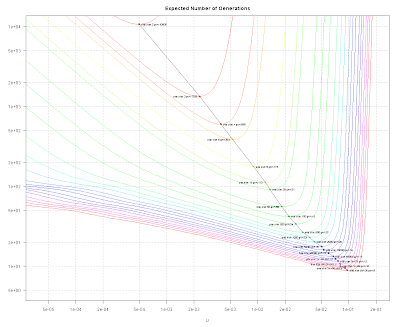
Obviously, the greater the size of the population for a fixed µ, the smaller the number of generations it takes to find the target. On the other hand, for a fixed population size, a similar rule for µ can't be given - one probably wants to keep the parent in the next generation, so µ has to be quite small for small populations, and can be bigger for great ones.

Here, the coloured lines represent the expected values of the number of generations for different sizes of population as a function of µ. At each curve, I added the minimal expected number - and I joined these minima by a black line. So, a population size of 200 results at best in 49 generation on average - and this minimum is reached for µ ~ 0.044.

But if you want to have a fast algorithm, you'd look at the number of queries, not the number of generations, i.e., the total number of children, or how often the fitness function has to be calculated:

(Yep, I like this pic :-) Here, you can see that for getting the best results, the size of the population is surprisingly small: 20 individuals. But though it takes over 325 generations on average to reach the target, the fitness value for only ~6514 individuals has to be calculated - that is, if you chose µ ~ 0.041.
Another interesting effect: for population sizes from 20 to 200, the optimal µ doesn't change very much, it's just a little bit over 0.04.

Of course, no one does these calculations before running the program: you write your weasel and play with it. But the natural behaviour of this algorithm will lead you to population sizes from 20 to 200, and a µ of 0.04 - 0.05.